Motion Detection Tutorial using OpenCV | Python
- Hackers Realm
- Oct 5, 2024
- 10 min read
Motion detection is a crucial feature in many modern applications, ranging from security surveillance systems to home automation and even robotics. It allows systems to sense movement in a video feed and respond accordingly, enhancing interactivity and security. In this tutorial, we'll explore how to implement a simple yet effective motion detection system using OpenCV, an open-source computer vision library that's widely used for image processing and video analysis.

With OpenCV, we can easily process video streams and analyze frame differences to detect changes over time, which signifies motion. Whether you're building a surveillance system that alerts you to intruders or simply experimenting with computer vision, understanding how to detect motion is a foundational skill. In this guide, we’ll take you through the basics of setting up OpenCV, processing video frames, and implementing a real-time motion detection algorithm.
By the end of this tutorial, you'll not only understand the core concepts behind motion detection but also be able to build a working Python program that uses OpenCV to identify movement in a video stream. So, let’s dive in and get started with creating your own motion detection system!
You can watch the video-based tutorial with step by step explanation down below.
Import Modules
import cv2
import numpy as np
import matplotlib.pyplot as plt
import imutils
import timecv2: The OpenCV library, used for image and video processing.
numpy (np): A library used for numerical operations, which is essential for manipulating image arrays.
matplotlib.pyplot (plt): Useful for plotting images and visualizing data.
imutils: A set of utility functions to make basic image processing tasks easier, like resizing or rotating.
time: This can be used to introduce delays or measure the time taken for different sections of your code, useful for performance analysis.
Load and Preprocess Image
Next we will load and preprocess the image.
# load and preprocess the image
def load_and_preprocess(image_path):
    image = cv2.imread(image_path)
    image = cv2.resize(image, (1280, 720))
    gray_image = cv2.cvtColor(image, cv2.COLOR_BGR2GRAY)
    return image, gray_image
The function load_and_preprocess(image_path) is designed to load an image from the given file path and perform some preprocessing steps to prepare it for further analysis.
cv2.imread(image_path):
This function reads an image from the specified image_path.
The image is loaded in color mode (BGR by default in OpenCV), meaning it retains all the color information from the original image.
The result is stored in the variable image.
cv2.resize(image, (1280, 720)):
The image is resized to a fixed resolution of 1280 (width) by 720 (height) pixels.
Resizing is important to standardize the input images, especially if you're working with images of different sizes. It helps in ensuring consistent processing across all images.
The resized image replaces the original one in the variable image.
cv2.cvtColor(image, cv2.COLOR_BGR2GRAY):
Converts the color image (image) from BGR (Blue, Green, Red) format to grayscale.
Grayscale images are simpler to process and require less computational power compared to color images, making them ideal for many image processing tasks.
The resulting grayscale image is stored in the variable gray_image.
return image, gray_image:
Returns both the resized color image (image) and the grayscale image (gray_image).
The color image might be useful for visualization purposes, while the grayscale version can be used for analysis, such as motion detection.
Next we will subtract the image to detect changes.
# subtract images
def subtract_images(image1, image2):
    diff = cv2.absdiff(image1, image2)
    _, thresh = cv2.threshold(diff, 50, 255, cv2.THRESH_BINARY)
    return diff, thresh
The function subtract_images(image1, image2) takes two images as input and calculates the difference between them to identify changes, such as movement or modifications.
cv2.absdiff(image1, image2):
cv2.absdiff() computes the absolute difference between the pixel values of two images, image1 and image2.
This function essentially subtracts each pixel value of image2 from the corresponding pixel value of image1, and takes the absolute value of the result. This way, it highlights the areas that are different between the two images.
The result is stored in diff, which is an image showing the differences between image1 and image2. Areas with no changes will be dark, while areas with changes will be highlighted.
cv2.threshold(diff, 50, 255, cv2.THRESH_BINARY):
Thresholding is used to convert the difference image (diff) into a binary image, where the pixels are either black (0) or white (255).
cv2.threshold() takes the following parameters:
diff: The input image that you want to threshold.
50: The threshold value. Any pixel value in diff greater than 50 will be set to 255 (white), while those less than or equal to 50 will be set to 0 (black).
255: The maximum value to be assigned to pixels that exceed the threshold.
cv2.THRESH_BINARY: This is the thresholding type, which creates a binary image with pixels either set to 0 or 255.
The result is stored in thresh. This binary image highlights regions where there are significant differences between the two input images. For example, moving objects between two consecutive frames would be represented as white areas.
return diff, thresh:
The function returns:
diff: The image representing the absolute differences between image1 and image2.
thresh: The binary thresholded image highlighting areas with significant changes.
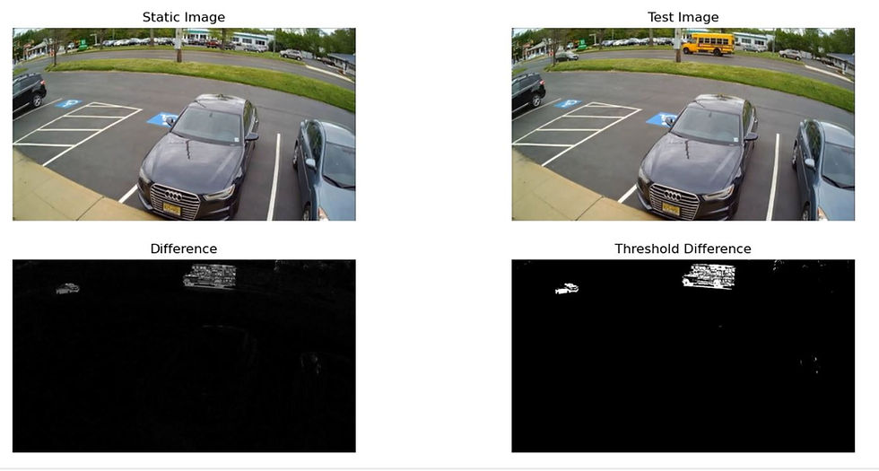
Next we will perform image processing to compare two images, static.png and test.png, in order to detect differences between them.
image_path1 = 'static.png'
image_path2 = 'test.png'

image1, gray_image1 = load_and_preprocess(image_path1)
image2, gray_image2 = load_and_preprocess(image_path2)

# subtract the images
diff, thresh = subtract_images(gray_image1, gray_image2)

# plot the images
plt.figure(figsize=(15, 7))

plt.subplot(2, 2, 1)
plt.title('Static Image')
plt.imshow(cv2.cvtColor(image1, cv2.COLOR_BGR2RGB))
plt.axis('off')

plt.subplot(2, 2, 2)
plt.title('Test Image')
plt.imshow(cv2.cvtColor(image2, cv2.COLOR_BGR2RGB))
plt.axis('off')

plt.subplot(2, 2, 3)
plt.title('Difference')
plt.imshow(diff, cmap='gray')
plt.axis('off')

plt.subplot(2, 2, 4)
plt.title('Threshold Difference')
plt.imshow(thresh, cmap='gray')
plt.axis('off')

plt.show()
Image Paths:
image_path1 and image_path2 contain the file paths for two images: static.png and test.png.
Load and Preprocess Images:
The function load_and_preprocess() is used to load and preprocess both images:
image1, gray_image1 = load_and_preprocess(image_path1): Loads the first image (static.png), resizes it to 1280x720, and converts it to grayscale.
image2, gray_image2 = load_and_preprocess(image_path2): Loads the second image (test.png), resizes it to 1280x720, and converts it to grayscale.
Subtract the Images:
diff, thresh = subtract_images(gray_image1, gray_image2):
The grayscale versions of the two images (gray_image1 and gray_image2) are compared using subtract_images().
This function computes the absolute difference between the two grayscale images (diff) and then thresholds this difference to create a binary image (thresh). This highlights regions with significant changes.
Plot the Images Using matplotlib:
A figure of size (15, 7) is created using plt.figure().
plt.subplot(2, 2, 1): Plots the original static image (image1).
The image is converted from BGR (OpenCV format) to RGB (matplotlib format) using cv2.cvtColor(image1, cv2.COLOR_BGR2RGB).
The title is set as "Static Image", and axes are turned off for better visualization.
plt.subplot(2, 2, 2): Plots the original test image (image2).
The same conversion from BGR to RGB is applied.
The title is set as "Test Image", and axes are turned off.
plt.subplot(2, 2, 3): Plots the difference image (diff).
The diff is displayed in grayscale using cmap='gray'.
The title is set as "Difference", and axes are turned off.
plt.subplot(2, 2, 4): Plots the thresholded difference image (thresh).
The binary image (thresh) is displayed in grayscale (cmap='gray').
The title is set as "Threshold Difference", and axes are turned off.
Display the Plot:
plt.show(): Displays all the images in a single figure window.
Next we will use dilation to enhance the thresholded image.
dilated_image = cv2.dilate(thresh, None, iterations=2)
plt.imshow(dilated_image, cmap='gray')
plt.axis('off')
plt.show()
cv2.dilate() is an image processing function used to expand white regions in a binary image.
thresh: This is the binary thresholded image, which highlights regions of difference between the two input images.
None: The kernel (structuring element) used for dilation. Passing None means OpenCV uses a default 3x3 kernel.
iterations=2: The number of times the dilation operation is applied to the image. More iterations result in a larger area of dilation.
dilated_image: The resulting image after dilation. Dilation is used to amplify the regions of change, making the detected areas more prominent. This is useful to fill in gaps and smooth the detected regions, especially when the thresholded image has small holes or noise.
plt.imshow(dilated_image, cmap='gray'): Displays the dilated image in grayscale.
plt.axis('off'): Hides the axis for a cleaner view of the image.
plt.show(): Displays the plot.
Dilation is particularly useful in motion detection to highlight and strengthen detected areas of movement.
After thresholding, the resulting image (thresh) may have small gaps or disconnected parts due to minor changes in lighting or noise. By applying dilation, the highlighted regions are expanded, helping to fill gaps and merge nearby contours. This results in a more cohesive detection of moving objects.
Next we will find contours in the dilated image, which helps in identifying the boundaries of objects detected as moving or changing.
cnts = cv2.findContours(dilated_image.copy(), cv2.RETR_EXTERNAL, cv2.CHAIN_APPROX_SIMPLE)
cnts = imutils.grab_contours(cnts)
Contours represent the boundaries of connected components in the binary image.
By finding the contours in the dilated_image, you can:
Identify moving objects in the scene by analyzing their boundaries.
Draw bounding boxes or other markers around detected objects for visualization.
Track object movement across frames.
cv2.findContours() is an OpenCV function that detects contours in a binary image.
dilated_image.copy():
A copy of the dilated image is passed as input. The copy() function is used to ensure that the original image is not modified during the contour-finding process.
cv2.RETR_EXTERNAL:
This parameter specifies the type of contours to retrieve.
cv2.RETR_EXTERNAL means only the external contours are retrieved, which is useful for identifying distinct objects rather than nested ones.
cv2.CHAIN_APPROX_SIMPLE:
This parameter specifies how contour points are stored.
cv2.CHAIN_APPROX_SIMPLE compresses horizontal, vertical, and diagonal segments, keeping only their end points. This helps reduce the memory usage by simplifying the contours.
imutils.grab_contours():
The function cv2.findContours() can return different results depending on the version of OpenCV you are using.
imutils.grab_contours() is a utility function from the imutils library that helps in extracting the correct set of contours from the result of cv2.findContours().
This makes the code more consistent across different OpenCV versions by ensuring cnts contains a list of contours that can be used further for analysis.
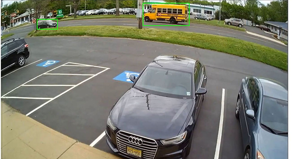
Next we will iterate over the detected contours and draws bounding boxes around the regions that have significant movement.
# iterate the contours
for c in cnts:
    if cv2.contourArea(c) < 700:
        continue

    # get the bounding box coordinates
    (x, y, w, h) = cv2.boundingRect(c)
    cv2.rectangle(image2, (x, y), (x+w, y+h), (0, 255, 0), 2)

cv2.imshow('test', image2)
cv2.waitKey(10000)
cv2.destroyAllWindows()
The loop iterates through each contour (c) in the list of contours (cnts), which was obtained using cv2.findContours().
cv2.contourArea(c):
This function calculates the area of the contour (c).
if cv2.contourArea(c) < 700::
If the area of the contour is smaller than 700, it is ignored by continuing to the next iteration.
This helps filter out small regions that may be noise or insignificant changes, thereby focusing only on larger, meaningful movements.
cv2.boundingRect(c):
This function computes the bounding rectangle for the contour (c).
It returns the coordinates of the top-left corner (x, y) and the width (w) and height (h) of the rectangle.
(x, y, w, h) are the bounding box coordinates, which help identify the position and size of the detected object.
cv2.rectangle():
Draws a rectangle on image2 around the detected movement.
(x, y) and (x+w, y+h) are the coordinates of the top-left and bottom-right corners of the bounding box.
(0, 255, 0) specifies the color of the rectangle in BGR format, which is green in this case.
2 specifies the thickness of the rectangle lines.
cv2.imshow('test', image2):
Displays the modified image2 with bounding boxes drawn around detected objects.
The window is titled 'test'.
cv2.waitKey(10000):
Waits for a key event for 10000 milliseconds (10 seconds).
If a key is pressed within this time, the window will close immediately.
cv2.destroyAllWindows():
Closes all OpenCV windows that were opened using cv2.imshow().
Test in Realtime / Video
Next we will implement motion detection in a video, either from a video file (test.mp4) or from a webcam, using OpenCV.
video_path = 'test.mp4'
# video_cap = cv2.VideoCapture(0) # capture from webcam
video_cap = cv2.VideoCapture(video_path)
static_frame = None

while True:
    success, frame = video_cap.read()
    if not success:
        break

    frame = cv2.resize(frame, (1280, 720))
    gray_frame = cv2.cvtColor(frame, cv2.COLOR_BGR2GRAY)

    if static_frame is None:
        static_frame = gray_frame
        continue

    # get the subtract frames
    diff, thresh = subtract_images(static_frame, gray_frame)
    dilated_image = cv2.dilate(thresh, None, iterations=2)

    # get contours
 cnts = cv2.findContours(dilated_image.copy(), cv2.RETR_EXTERNAL, 		       cv2.CHAIN_APPROX_SIMPLE)
    cnts = imutils.grab_contours(cnts)

    # iterate the contours
    for c in cnts:
        if cv2.contourArea(c) < 700:
            continue

        # get the bounding box coordinates
        (x, y, w, h) = cv2.boundingRect(c)
        cv2.rectangle(frame, (x, y), (x+w, y+h), (0, 255, 0), 2)

    cv2.imshow("Motion Detection", frame)

    # exit if any key is pressed
    if cv2.waitKey(1) & 0xFF != 255:
        break
    time.sleep(0.1)

video_cap.release()
cv2.destroyAllWindows()
Video Capture Setup:
video_path = 'test.mp4': Path to the video file to be used for motion detection.
video_cap = cv2.VideoCapture(0) (commented out): This line, if uncommented, would allow capturing video directly from a webcam. The 0 refers to the default camera device.
video_cap = cv2.VideoCapture(video_path): Initializes a VideoCapture object (video_cap) to read from the video file specified by video_path.
Initial Frame Setup:
static_frame = None: Used to store the first frame of the video, which will act as a reference for motion detection. It is initially set to None.
Processing Each Frame:
while True:: A loop that processes each frame of the video.
success, frame = video_cap.read(): Reads a frame from the video.
success indicates whether reading the frame was successful.
frame contains the image of the current frame.
if not success:: If no frame is returned (end of video), the loop breaks.
Preprocess the Frame:
frame = cv2.resize(frame, (1280, 720)): Resizes the frame to 1280x720 pixels.
gray_frame = cv2.cvtColor(frame, cv2.COLOR_BGR2GRAY): Converts the frame to grayscale for easier processing.
Initialize the Static Frame:
if static_frame is None:: If static_frame is not yet set (i.e., it’s the first iteration of the loop), it is assigned the current gray_frame.
continue: Skips the rest of the loop to avoid comparing the first frame with itself.
Frame Subtraction and Dilation:
subtract_images(static_frame, gray_frame): Computes the absolute difference between the static_frame (reference frame) and the current gray_frame. It returns diff and thresh.
cv2.dilate(thresh, None, iterations=2): Applies dilation to enhance the thresholded image (thresh) to make detected areas more prominent.
Finding Contours:
cv2.findContours() finds the external contours in the dilated_image.
imutils.grab_contours() extracts the list of contours from the result of cv2.findContours().
Iterate and Draw Bounding Boxes:
The loop iterates over each contour (c).
if cv2.contourArea(c) < 700: skips any contour whose area is smaller than 700 to ignore small, insignificant movements.
cv2.boundingRect(c) finds the bounding box for the contour.
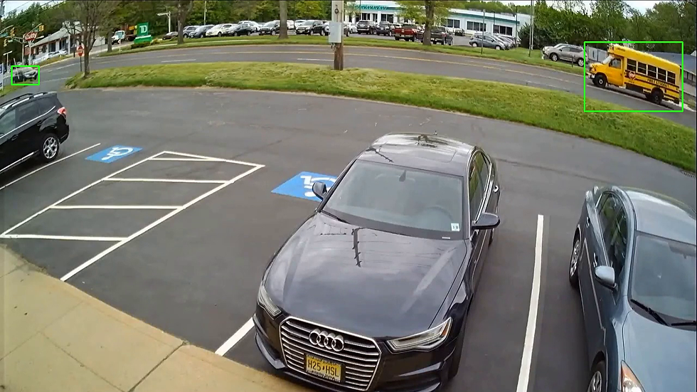
cv2.rectangle() draws a green bounding box around the detected movement on the original frame.
Display the Frame with Detected Motion:
Next display the frame with the bounding boxes drawn around detected areas of motion in a window titled "Motion Detection".
Exit Condition:
cv2.waitKey(1) waits for a key event for 1 millisecond. If a key is pressed (i.e., != 255), the loop breaks, ending the video playback.
time.sleep(0.1) introduces a 0.1-second delay between frames to slow down the playback for better visualization.
Release Resources:
video_cap.release(): Releases the video capture object.
cv2.destroyAllWindows(): Closes all OpenCV windows.
Final Thoughts
Motion detection using OpenCV is a powerful technique that allows you to identify and track movement in a video stream, whether from a file or a live feed.
This tutorial covered the fundamental steps—from loading and preprocessing images to using frame differencing, thresholding, and dilation to detect motion effectively.
By understanding how to locate contours and filter noise, you can customize this basic approach for various real-world applications, such as security surveillance, activity monitoring, or automated video analysis.
We encourage you to experiment further, optimize the code to suit your specific requirements, and explore advanced motion detection techniques to make your applications smarter and more responsive. Whether you're just getting started or looking to expand your existing knowledge, OpenCV opens up a world of possibilities for computer vision projects.
Get the project notebook from here
Thanks for reading the article!!!
Check out more project videos from the YouTube channel Hackers Realm

Kommentare