Multi-label classification is a machine learning task where each instance (or data point) is associated with multiple labels simultaneously. Unlike traditional classification tasks where each instance is assigned to a single label, multi-label classification deals with scenarios where the categories are not mutually exclusive. This means an instance can belong to one or more classes or categories at the same time.
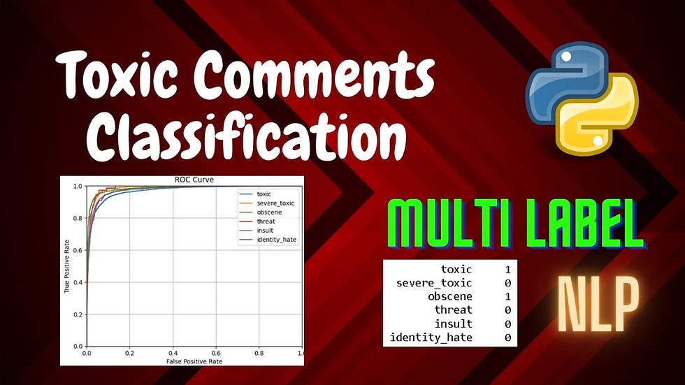
The challenge in multi-label classification lies in predicting a set of labels for each instance accurately, often requiring specialized algorithms and evaluation metrics that can handle multiple predictions per instance.
In this tutorial, we will analyse large number of Wikipedia comments which have been labeled by human raters for toxic behavior using multi-label classification.
You can watch the video-based tutorial with step by step explanation down below.
Import Modules
import pandas as pd
import numpy as np
import re
import matplotlib.pyplot as plt
import seaborn as sns
import nltk
from nltk.corpus import stopwords
from nltk.stem.snowball import SnowballStemmer

from sklearn.model_selection import train_test_split
from sklearn.feature_extraction.text import TfidfVectorizer
from sklearn.pipeline import Pipeline
from sklearn.multiclass import OneVsRestClassifier
from sklearn.linear_model import LogisticRegression
from sklearn.naive_bayes import MultinomialNB
from sklearn.metrics import roc_auc_score, accuracy_score, roc_curve, classification_report

import warnings
warnings.filterwarnings('ignore')
pandas - used to perform data manipulation and analysis.
numpy - provides support for arrays, matrices, and a variety of mathematical functions to operate on these data structures.
re - provides support for regular expressions, which are patterns used for matching and manipulating strings.
matplotlib.pyplot - used for creating static, animated, and interactive visualizations in Python. pyplot is a module within Matplotlib that provides a MATLAB-like interface.
seaborn - provides a high-level interface for creating attractive and informative statistical graphics. Seaborn is particularly useful for visualizing relationships between variables, exploring distributions, and presenting complex statistical analyses.
nltk - suite of libraries and programs for symbolic and statistical natural language processing (NLP) in Python.
scikit-learn - machine learning library in Python that provides tools for model training, evaluation, and preprocessing.
warnings - used to control and suppress warning messages that may be generated by the Python interpreter or third-party libraries during the execution of a Python program.
Import Data
Next we will read the data from the csv file .
df = pd.read_csv('train.csv')
df.head()
pd.read_csv('train.csv'): This function reads the CSV file into a pandas DataFrame. The file train.csv should be in the same directory as your script or notebook, or you need to provide the full path to the file.
df.head(): This method returns the first 5 rows of the DataFrame by default. It allows you to inspect the top of your dataset to understand its structure, including the column names and some initial data.
Next we will see the statistical summary of the DataFrame.
# dataset stats
df.describe()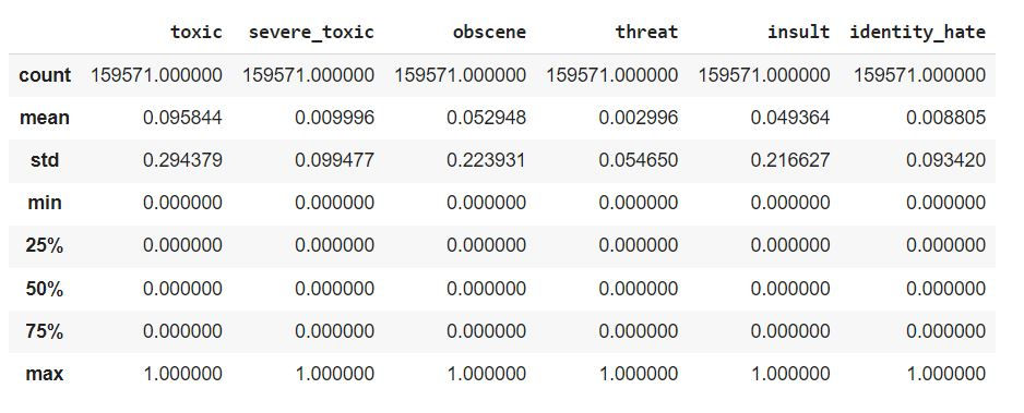
The df.describe() function provides a statistical summary of your DataFrame.This summary includes the following statistics for each numerical column in your dataset:
Count: The number of non-null (non-missing) values in each column.
Mean: The average of the values in each column.
Std: The standard deviation, which measures the spread of the data.
Min: The minimum value in each column.
25%: The 25th percentile (also known as the first quartile), which means that 25% of the data falls below this value.
50%: The 50th percentile (also known as the median), which means that 50% of the data falls below this value.
75%: The 75th percentile (also known as the third quartile), which means that 75% of the data falls below this value.
Max: The maximum value in each column.
This summary is useful for getting an initial understanding of the distribution of your data, identifying potential outliers, and understanding the range and central tendency of each numerical column.
Next we will get some information of the dataframe.
# dataset info
df.info()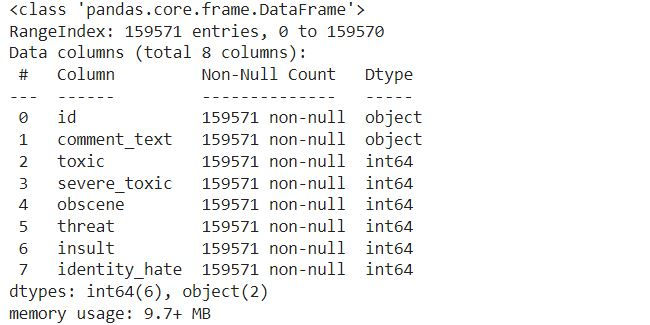
The df.info() function provides a concise summary of your DataFrame, which includes the following information:
Index: The number of rows in the DataFrame.
Column names: The names of all the columns in the DataFrame.
Non-null count: The number of non-null (non-missing) values in each column.
Dtype: The data type of each column (e.g., int64, float64, object).
This information is useful for understanding the structure of your DataFrame, identifying columns with missing data, and verifying that the data types are as expected.
Next we will identify if we have missing values.
# check for null values
df.isnull().sum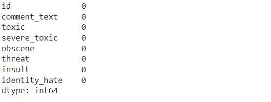
The df.isnull().sum() function is used to identify the number of missing (null) values in each column of your DataFrame. Here’s what it does:
df.isnull(): This part of the code creates a DataFrame of the same shape as df, where each cell contains True if the value is missing (null) and False otherwise.
sum(): Summing over the True values in each column (where True is treated as 1 and False as 0) gives the total count of missing values in each column.
The result is a Series that lists the columns and the corresponding number of missing values.
Next we will check the number of records in the dataframe.
len(df)159571
The len(df) function returns the number of rows in your DataFrame df.
Exploratory Data Analysis
First we will select only label columns.
x = df.iloc[:, 2:].sum() # take only label columns
x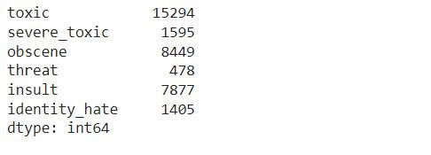
df.iloc[:, 2:]: This part of the code selects all rows (:) and all columns starting from the 3rd column (index 2) to the last column. The assumption here is that the first two columns are not label columns and that the label columns start from the 3rd column onward.
sum(): This sums the values in each selected column. Since it is assumed that the label columns contain binary values (e.g., 0 and 1), the sum for each column would represent the total number of instances where the label is present (i.e., the count of 1s in each column).
The result, stored in x, is a Series where each index corresponds to a label column and each value is the total count of that label across all rows.
Next we will select the label columns and sum it column-wise.
rowsums = df.iloc[:, 2:].sum(axis=1) # take label columns and sum it column wise
rowsums
df.iloc[:, 2:]: This selects all rows (:) and all columns starting from the 3rd column (index 2) to the last column. These columns are assumed to be the label columns.
sum(axis=1): This sums the values across columns for each row. The axis=1 argument specifies that the sum should be calculated across columns (horizontally) for each row.
The result, stored in rowsums, is a Series where each entry represents the total number of labels present (i.e., the number of 1s) for each row in the dataset.
Next we will see the row wise sum.
no_label_count = 0
for i, count in rowsums.items():
	if count==0:
		no_label_count += 1
print('Total number of comments:', len(df))
print('Total number of comments without labels:', no_label_count) 			print('Total labels:', x.sum())
Total number of comments: 159571
Total number of comments without labels: 143346
Total labels: 35098
Initialize no_label_count = 0: This variable is used to count the number of rows (comments) that have no labels (i.e., all label columns are 0).
Loop through rowsums:
for i, count in rowsums.items(): This iterates over each row's index i and its corresponding sum of labels count from the rowsums Series.
if count == 0: Checks if the sum of labels for that row is 0, meaning the comment has no associated labels.
no_label_count += 1: If a row has no labels, it increments the no_label_count by 1.
Print statements:
print('Total number of comments:', len(df)): Outputs the total number of comments (rows) in the dataset.
print('Total number of comments without labels:', no_label_count): Outputs the total number of comments that have no labels.
print('Total labels:', x.sum()): Outputs the total number of labels across all comments, which is the sum of all values in x (which is the sum of each label column across all rows).
Next we will create a bar plot to visualize the count of each label in the dataset.
plt.figure(figsize=(6, 4))
ax = sns.barplot(x=x.index, y=x.values, alpha=0.8, palette=['tab:blue', 'tab:orange', 'tab:green', 'tab:brown', 'tab:red', 'tab:grey'])
plt.title('Label Counts')
plt.ylabel('Count')
plt.xlabel('Label')

plt.show()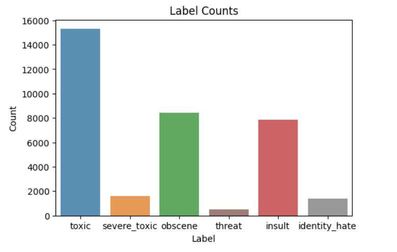
plt.figure(figsize=(6, 4)): Initializes a new figure with a size of 6 inches by 4 inches. This sets up the canvas for the plot.
ax = sns.barplot(x=x.index, y=x.values, alpha=0.8, palette=['tab:blue', 'tab:orange', 'tab:green', 'tab:brown', 'tab:red', 'tab:grey']):
x=x.index: Sets the x-axis to the labels (column names) from x.
y=x.values: Sets the y-axis to the counts of each label from x.
alpha=0.8: Sets the transparency level of the bars.
palette=['tab:blue', 'tab:orange', 'tab:green', 'tab:brown', 'tab:red', 'tab:grey']: Specifies a color palette for the bars.
plt.title('Label Counts'): Sets the title of the plot to "Label Counts".
plt.ylabel('Count'): Labels the y-axis as "Count".
plt.xlabel('Label'): Labels the x-axis as "Label".
plt.show(): Displays the plot.
Next we will create a count plot to visualize the distribution of the number of labels per comment.
plt.figure(figsize=(6, 4))
ax = sns.countplot(x=rowsums.values, alpha=0.8, palette=['tab:blue', 'tab:orange', 'tab:green', 'tab:brown', 'tab:red', 'tab:grey'])
plt.title('Labels per Comment')
plt.ylabel('# of Occurences')
plt.xlabel('# of Labels')
plt.show()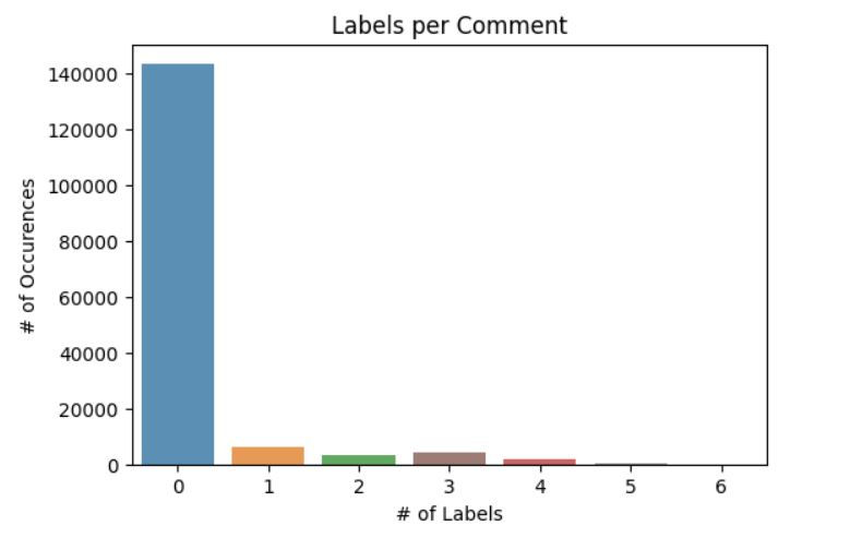
plt.figure(figsize=(6, 4)): Initializes a new figure with a size of 6 inches by 4 inches.
ax = sns.countplot(x=rowsums.values, alpha=0.8, palette=['tab:blue', 'tab:orange', 'tab:green', 'tab:brown', 'tab:red', 'tab:grey']):
x=rowsums.values: Sets the x-axis to the values of rowsums, which represent the number of labels per comment.
alpha=0.8: Sets the transparency level of the bars.
palette=['tab:blue', 'tab:orange', 'tab:green', 'tab:brown', 'tab:red', 'tab:grey']: Specifies a color palette for the bars.
plt.title('Labels per Comment'): Sets the title of the plot to "Labels per Comment".
plt.ylabel('# of Occurences'): Labels the y-axis as "# of Occurrences", indicating the number of comments for each number of labels.
plt.xlabel('# of Labels'): Labels the x-axis as "# of Labels", showing the number of labels assigned to each comment.
plt.show(): Displays the plot.
Data Preprocessing
First we will first remove columns that are not required.
df = df.drop(columns=['id'], axis=1)
df.head()
df.drop(columns=['id'], axis=1): This specifies that you want to drop the column named 'id' from the DataFrame. The axis=1 argument indicates that you're removing a column (not a row).
The df.head() command will then display the first few rows of the updated DataFrame without the 'id' column.
Next we will preprocess the text.
# remove stopwords
stopwords = set(stopwords.words('english'))

def remove_stopwords(text):
    no_stopword_text = [w for w in text.split() if not w in stopwords]
    return " ".join(no_stopword_text)

def clean_text(text):
    text = text.lower()
    text = re.sub(r"what's", "what is ", text)
    text = re.sub(r"\'s", " ", text)
    text = re.sub(r"\'ve", " have ", text)
    text = re.sub(r"can't", "can not ", text)
    text = re.sub(r"n't", " not ", text)
    text = re.sub(r"i'm", "i am ", text)
    text = re.sub(r"\'re", " are ", text)
    text = re.sub(r"\'d", " would ", text)
    text = re.sub(r"\'ll", " will ", text)
    text = re.sub(r"\'scuse", " excuse ", text)
    text = re.sub('\W', ' ', text)
    text = re.sub('\s+', ' ', text)
    text = text.strip(' ')
    return text

# stemming
stemmer = SnowballStemmer('english')
def stemming(sentence):
    stemmed_sentence = ""
    for word in sentence.split():
        stemmed_word = stemmer.stem(word)
        stemmed_sentence += stemmed_word + " "

    stemmed_sentence = stemmed_sentence.strip()
    return stemmed_sentence
Removing Stopwords:
stopwords = set(stopwords.words('english')): Retrieves a set of English stopwords from the NLTK library, which are commonly used words that are often removed during text preprocessing.
remove_stopwords(text): This function takes a string text and removes all stopwords from it. It splits the text into words, filters out the stopwords, and then joins the remaining words back into a string.
Text Cleaning:
clean_text(text): This function performs several text normalization tasks:
Converts the text to lowercase.
Expands contractions (e.g., "can't" to "can not").
Replaces common contractions and special characters with their expanded forms or spaces.
Removes non-alphanumeric characters and extra spaces.
Strips leading and trailing spaces.
Stemming:
stemmer = SnowballStemmer('english'): Initializes the Snowball Stemmer for English, which is used for reducing words to their root form.
stemming(sentence): This function stems each word in the provided sentence. It splits the sentence into words, applies stemming to each word, and then reconstructs the sentence from the stemmed words.
Next we will apply the preprocessing functions to the comment_text column in your DataFrame df.
# preprocess the comment
df['comment_text'] = df['comment_text'].apply(lambda x: remove_stopwords(x))
df['comment_text'] = df['comment_text'].apply(lambda x: clean_text(x))
df['comment_text'] = df['comment_text'].apply(lambda x: stemming(x))
df.head()
Remove Stopwords: the remove_stopwords function to each comment in the comment_text column, removing common English stopwords that are not likely to contribute to the meaning of the text.
Clean Text: the clean_text function to each comment, normalizing the text by converting it to lowercase, expanding contractions, removing special characters, and eliminating extra spaces.
Apply Stemming: the stemming function to each comment, reducing words to their root form. This standardizes different forms of a word to a common base, which is useful in reducing dimensionality in text data.
Finally, the df.head() command displays the first few rows of the updated DataFrame, showing the preprocessed comment_text column.
Next we will split the DataFrame into input features (X) and output labels (y).
# split input and output
X = df['comment_text']
y = df.drop(columns=['comment_text'], axis=1)
X = df['comment_text']: This line selects the comment_text column from the DataFrame df and assigns it to X. This will be the input data used for training the model, consisting of the preprocessed text comments.
y = df.drop(columns=['comment_text'], axis=1): This line drops the comment_text column from the DataFrame and assigns the remaining columns to y. These remaining columns represent the labels for the multi-label classification task. Each row in y corresponds to the set of labels associated with a comment in X.
Next we will split the data for training and testing.
# split data for training and testing
X_train, X_test, y_train, y_test = train_test_split(X, y, test_size=0.2, random_state=42)train_test_split:
X: The input features (preprocessed comment_text).
y: The output labels (the remaining columns that represent the multi-label classifications).
test_size=0.2: Specifies that 20% of the data should be used for testing, while the remaining 80% is used for training.
random_state=42: Ensures that the data split is reproducible. Using the same random_state value will result in the same split each time the code is run.
Resulting Variables:
X_train: Contains 80% of the comments for training.
X_test: Contains 20% of the comments for testing.
y_train: Contains the corresponding labels for the training comments.
y_test: Contains the corresponding labels for the testing comments.
Next we will train a machine learning model using a pipeline, make predictions, and then evaluate the model’s performance on the test data.
def run_pipeline(pipeline, X_train, X_test, y_train, y_test):
    # train model
    pipeline.fit(X_train, y_train)
    # predict from model
    predictions = pipeline.predict(X_test)
    pred_probs = pipeline.predict_proba(X_test)
    # print metrics
    print('roc_auc:', roc_auc_score(y_test, pred_probs))
    print('accuracy:', accuracy_score(y_test, predictions))
    print('classification report')
print(classification_report(y_test, predictions, target_names=y_train.columns))pipeline.fit(X_train, y_train): The pipeline is fitted to the training data (X_train and y_train). This step involves training the model using the training dataset.
pipeline.predict(X_test): Predicts the labels for the test set (X_test).
pipeline.predict_proba(X_test): Predicts the probability estimates for each label in the test set. This is particularly useful for computing metrics like ROC-AUC.
Next compute and print the ROC-AUC score, a metric that evaluates the performance of the model across all possible classification thresholds.
Next compute and print the accuracy of the model, which is the ratio of correctly predicted instances to the total instances.
Next print a detailed classification report, which includes precision, recall, and F1-score for each label. The target_names argument is used to display the actual label names in the report.
Next we will create two pipelines, one using a Naive Bayes model (NB_pipeline) and the other using a Logistic Regression model (LR_pipeline).
NB_pipeline = Pipeline([     ('tfidf', TfidfVectorizer(stop_words='english')),     ('nb_model', OneVsRestClassifier(MultinomialNB(), n_jobs=-1)) ])

LR_pipeline = Pipeline([     ('tfidf', TfidfVectorizer(stop_words='english')),     ('nb_model', OneVsRestClassifier(LogisticRegression(), n_jobs=-1))])
Naive Bayes Pipeline (NB_pipeline):
TfidfVectorizer(stop_words='english'): This step transforms the input text data into a TF-IDF matrix, while also removing English stopwords.
OneVsRestClassifier(MultinomialNB(), n_jobs=-1): This step trains a Multinomial Naive Bayes model using the One-vs-Rest strategy for multi-label classification. The n_jobs=-1 parameter allows the computation to run in parallel, utilizing all available processors.
Logistic Regression Pipeline (LR_pipeline):
TfidfVectorizer(stop_words='english'): Like in the Naive Bayes pipeline, this step converts the text data into a TF-IDF matrix and removes English stopwords.
OneVsRestClassifier(LogisticRegression(), n_jobs=-1): This step trains a Logistic Regression model using the One-vs-Rest strategy for multi-label classification, also utilizing parallel computation with n_jobs=-1.
Next we will run the NB_pipeline on the training and test data and evaluate its performance.
run_pipeline(NB_pipeline, X_train, X_test, y_train, y_test)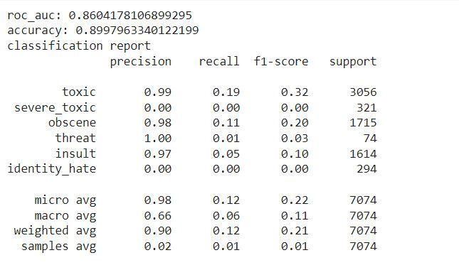
This will train the Naive Bayes model on the training data (X_train, y_train), make predictions on the test data (X_test), and then print the ROC-AUC score, accuracy, and classification report based on the test labels (y_test).
Next we will evaluate the Logistic Regression pipeline (LR_pipeline).
run_pipeline(LR_pipeline, X_train, X_test, y_train, y_test)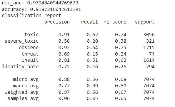
Train the Logistic Regression model on the training data (X_train, y_train).
Make predictions on the test data (X_test).
Print the ROC-AUC score, accuracy, and classification report for the model's performance on the test labels (y_test).
After running this, you'll see the evaluation metrics, which will help you understand how well the Logistic Regression model performs in comparison to the Naive Bayes model.
Test Prediction
First we will extract the names of the label columns from the y_train DataFrame.
labels = y_train.columns.values
labels
array(['toxic', 'severe_toxic', 'obscene', 'threat', 'insult', 'identity_hate'], dtype=object)
y_train.columns.values: This retrieves the column names from the y_train DataFrame as a NumPy array. Since y_train contains the labels for your multi-label classification task, this array will contain the names of those labels.
labels: This variable now holds the array of label names.
When you run labels, it will display the array of all label names in y_train.
Next we will randomly select one comment from the X_test dataset.X_test.sample(1).values[0].
X_test.sample(1).values[0]'hello dick wikipedia fuckwhit ban'
X_test.sample(1): This randomly selects one sample (in this case, one comment) from the X_test DataFrame.
.values: This converts the selected sample into a NumPy array.
[0]: Since sample(1) returns a DataFrame with a single row, this indexing extracts the text content from that row as a string.
Next we will process a given sentence and predict its labels using the Logistic Regression pipeline (LR_pipeline).
sentence = 'hello dick wikipedia fuckwhit ban'
stemmed_sentence = stemming(sentence)
results = LR_pipeline.predict([stemmed_sentence])[0]
for label, result in zip(labels, results):
    print("%14s %5s" % (label, result))
toxic 1
severe_toxic 0
obscene 1
threat 0
insult 0
identity_hate 0
The stemming function is applied to the input sentence to reduce each word to its base or root form. This preprocessing step helps in standardizing the input before it is fed into the model.
The preprocessed sentence is passed through the Logistic Regression pipeline (LR_pipeline) to predict the labels. The result is a binary array indicating the presence (1) or absence (0) of each label.
The labels and the corresponding prediction results are iterated over and printed in a formatted manner, showing each label and whether it was predicted as present (1) or absent (0).
This output indicates which labels the Logistic Regression model predicts for the given sentence. In this case, it might predict "toxic," "obscene," and "insult" as present.
Next we will process another sentence and predict its labels using the Logistic Regression pipeline (LR_pipeline).
sentence = 'hello how are you doing'
stemmed_sentence = stemming(sentence)
results = LR_pipeline.predict([stemmed_sentence])[0]
for label, result in zip(labels, results):
    print("%14s %5s" % (label, result))
toxic 0
severe_toxic 0
obscene 0
threat 0
insult 0
identity_hate 0
The stemming function will reduce each word in the sentence to its base or root form. However, since this sentence contains common words that might not change much during stemming, the output might be quite similar to the input.
The Logistic Regression pipeline (LR_pipeline) predicts labels for the stemmed sentence. The output, results, will be a binary array indicating whether each label is present (1) or not (0).
The output suggests that the model predicts none of the negative labels (like "toxic" or "insult") as present for this sentence.
ROC Curve
Next we will plot the ROC curves for each label using the Logistic Regression pipeline (LR_pipeline).
def plot_roc_curve(test_labels, predict_prob):
    fpr, tpr, thresholds = roc_curve(test_labels, predict_prob)
    plt.plot(fpr, tpr)
    plt.xlim([0.0, 1.0])
    plt.ylim([0.0, 1.0])
    plt.title('ROC Curve')
    plt.xlabel('False Positive Rate')
    plt.ylabel('True Positive Rate')
    plt.grid(True)
    plt.legend(labels)

def plot_pipeline_roc_curve(pipeline, X_train, X_test, y_train, y_test):
    for label in labels:
        pipeline.fit(X_train, y_train[label])
        pred_probs = pipeline.predict_proba(X_test)[:, 1]
        plot_roc_curve(y_test[label], pred_probs)

plot_pipeline_roc_curve(LR_pipeline, X_train, X_test, y_train, y_test)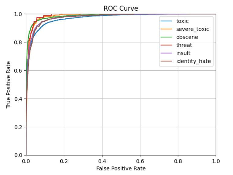
roc_curve(test_labels, predict_prob): Calculates the False Positive Rate (FPR) and True Positive Rate (TPR) at different thresholds for the given label.
plt.plot(fpr, tpr): Plots the ROC curve, which is a plot of TPR (sensitivity) against FPR.
plt.xlim([0.0, 1.0]) and plt.ylim([0.0, 1.0]): Sets the x-axis and y-axis limits to the range [0, 1].
plt.title, plt.xlabel, plt.ylabel: Adds a title and labels to the plot.
plt.grid(True): Adds a grid to the plot for better readability.
plt.legend(labels): Adds a legend with the label names (this might need adjustment since it adds all labels, not just the one being plotted).
for label in labels:: Iterates over each label in the dataset.
pipeline.fit(X_train, y_train[label]): Trains the pipeline model on the training data for the current label.
pred_probs = pipeline.predict_proba(X_test)[:, 1]: Predicts the probability of the positive class (label present) for the test data.
plot_roc_curve(y_test[label], pred_probs): Plots the ROC curve for the current label using the plot_roc_curve function.
This line calls plot_pipeline_roc_curve to generate and display ROC curves for all labels using the Logistic Regression pipeline.
Final Thoughts
Multi-label classification is a complex yet fascinating area of machine learning where each instance in the dataset can be assigned multiple labels, as opposed to the traditional single-label classification.
Often, labels are not equally represented, leading to challenges in training models that perform well across all labels. Special techniques like re-sampling, cost-sensitive learning, or thresholding are sometimes needed.
Standard metrics like accuracy or ROC-AUC must be adapted for multi-label settings. Metrics such as Hamming loss, Jaccard index, and subset accuracy are commonly used to evaluate performance in multi-label classification.
Multi-label classification is a powerful tool for solving real-world problems where each instance can belong to multiple categories simultaneously. While it introduces additional complexity compared to single-label classification, the development of specialized techniques and models has made it possible to address these challenges effectively. As data grows in both size and complexity, the importance and applicability of multi-label classification will continue to expand.
Get the project notebook from here
Thanks for reading the article!!!
Check out more project videos from the YouTube channel Hackers Realm

Comments